Code
library(tidyverse)
library(here)
library(ggthemes)
library(scales)
library(lubridate)
library(knitr)
library(gt)library(tidyverse)
library(here)
library(ggthemes)
library(scales)
library(lubridate)
library(knitr)
library(gt)Food insecurity remain a pervasive challenge in Tanzania, with approximately 40% of households lacking an adequate diet (Santalucia and Sibhatu 2023). A significant portion of the population relies heavily on diets dominated by staples, often lacking essential nutrient-rich foods (Ignowski et al. 2023). Notably, up to 65% of Tanzania’s population works in agriculture, making the dietary choices highly vulnerable to climatic shifts, seasonality, and price fluctuations (Randell et al. 2022). While national surveys frequently capture how a households substitutes diverse, nutrient-dense foods with cheaper staples during a lean season (Ignowski et al. 2023), it remains largely obscured how these nutritional compromises are distributed. In this study, I map the seasonality of food scarcity, their drivers, and track the short-term coping strategies.
This study utilizes data from the Tanzanian National Panel Survey (NPS), a nationally representative survey implemented by the Tanzanian National Bureau of Statistics with support from the World Bank’s Living Standards Measurement Study - Integrated Surveys on Agriculture (LSMS-ISA) project. The analysis relies on a combined, unified panel dataset spanning four survey waves (NPSY1 through NPSY4). By leveraging the Uniform Panel Household Identifier (UPHI), the study tracks the same households across multiple years, providing a longitudinal perspective on how specific families navigate repeated periods of food scarcity. The data is anonymized and available for public use.
To map the incidence of shocks and the resulting coping mechanisms, this study constructs a focused set of descriptive variables drawn from the survey’s household food security modules upd4_hh_h:
Seasonal shocks and vulnerability: Acute food scarcity is identified using a 12-month retrospective indicator (hh_08), which records whether a household faced a situation where they did not have enough food. The dataset provides high-resolution temporal data (hh_09_01 through hh_11_36) capturing the exact months and years these shortages occurred, allowing for the precise mapping of seasonal lean periods.
Shock typologies: To differentiate between environmental and economic stressors, the analysis utilizes categorical variables (hh_12_1 to hh_12_3) that record the top three self-reported causes of the experienced food shortages in the corresponding order (e.g., droughts, floods, crop pests, or localized price spikes).
Short-term coping mechanisms: The analysis incorporates 7-day recall variables measuring food-related anxiety (hh_01) and the frequency, in days, that households resorted to negative dietary coping strategies (hh_02_1 through hh_02_8).
This study employs a rigorous descriptive approach as opposed to econometric modelling to visualize the lived realities of food scarcity. The analysis flows in three categories:
Temporal mapping: To establish the seasonal chronology of food shortages, the study aggregates the month-by-month shortage indicators to construct seasonal frequency distributions. The trend is visualized through a column chart. The peak vulnerability windows are visualized in a column chart that shows the trend throughout the years.
Typology frequencies: To identify the dominant causes of food scarcity throughout the calendar year, self-reported shock data from all survey rounds (NPSY1–NPSY4) are pooled by calendar month (January through December).
Within each month, reported shortage causes (hh_12_1 through hh_12_3) are grouped into their respective rank categories: Primary Cause, Secondary Cause, and Tertiary Cause.
Frequency counts are calculated across the pooled dataset to identify the single most prevalent (modal) driver of scarcity for each ranking category within every calendar month.
This modal aggregation generated a synthesized 12-month profile (presented in Table 1).
To evaluate how households adapt in the short term when faced with food deficits, the analysis examines 7-day recall food security indicators (hh_01 for food anxiety and hh_02_1 through hh_02_6 for specific coping behaviors) across panel waves (Waves 2, 3, and 4).
I calculate the percentage of households adopting individual dietary coping mechanisms—ranging from dietary quality adjustments (relying on less preferred foods) to quantitative rationing (reducing portion sizes, skipping meals) and severe distress behaviors (adults restricting intake for children, full-day fasting).
Standardized severity weights are applied to the 7-day frequency of these coping behaviors to compute household-level reduced Coping Strategies Index (rCSI) scores (Maxwell, Caldwell, and Langworthy 2008), tracking mean population-level distress and adaptation trajectories across successive panel rounds (Table 2).
The aggregated monthly reports of household food shortages across NPS survey rounds demonstrate a pronounced, recurring annual cycle.
# 1. Load Raw Dataset with col_types = cols(.default = "c") to prevent parsing warnings
raw_data <- read_csv(
  here::here("data/raw/upd4_hh_h.csv"),
  col_types = cols(.default = "c")
)

# 2. Reshape & Filter Temporal Scarcity Data
temp_mapping <- raw_data |>
  select(
    UPHI, round, hh_08,
    starts_with("hh_09"),
    starts_with("hh_10"),
    starts_with("hh_11")
  ) |>
  filter(!is.na(hh_08) & hh_08 %in% c("YES", "Yes", "1")) |>
  rename(
    household_id = UPHI,
    wave = round,
    experienced_shortage_12m = hh_08
  ) |>
  pivot_longer(
    cols = starts_with("hh_"),
    names_to = "shortage_period_code",
    values_to = "shortage_reported"
  ) |>
  filter(!is.na(shortage_reported) & !shortage_reported %in% c("NO", "No", "0", "FALSE")) |>
  select(household_id, wave, shortage_period_code)

# Ensure directory exists before writing
dir.create(here::here("data/processed"), recursive = TRUE, showWarnings = FALSE)

write_csv(temp_mapping, here::here("data/processed/temporal-mapping-data.csv"))

# 3. Load Data Dictionary (adjust path to "data/raw/" if that's where dictionary.csv lives)
dict_path <- here::here("data/processed/dictionary.csv")
# dict_path <- here::here("data/raw/dictionary.csv") # <-- Use this if stored in raw/

dict <- read_csv(dict_path, col_types = cols(.default = "c"))

# 4. Map Dates from Variable Descriptions
date_lookup <- dict |>
  filter(str_detect(variable_name, "^hh_(09|10|11)")) |>
  mutate(
    year  = str_extract(description, "\\d{4}"),
    month = str_extract(description, "(?<=\\()[A-Za-z]+(?=\\))"),
    date  = dmy(paste("01", month, year)),
    date_label = format(date, "%b %Y")
  ) |>
  select(variable_name, date, date_label)

# 5. Merge Lookup Table with Processed Long Dataframe
temp_mapping_formatted <- temp_mapping |>
  inner_join(date_lookup, by = c("shortage_period_code" = "variable_name")) |>
  mutate(year = year(date))

# 6. Aggregate Monthly Frequencies Chronologically
seasonal_economic_dist <- temp_mapping_formatted |>
  group_by(date, year, date_label) |>
  summarize(total_reports = n(), .groups = "drop") |>
  arrange(date) |>
  mutate(pct_share = (total_reports / sum(total_reports)) * 100)

# 7. Plot with Economist Theme & Palette
p_econ <- ggplot(seasonal_economic_dist, aes(x = date, y = total_reports)) +
  geom_col(aes(fill = factor(year)), width = 25, show.legend = TRUE) +
  scale_fill_manual(
    values = c(
      "2009" = "#014d64",
      "2010" = "#00887d",
      "2011" = "#01a2d9",
      "2012" = "#6794a7",
      "2013" = "#7ad2f6"
    ),
    name = "Year"
  ) +
  scale_x_date(
    date_breaks = "1 month",
    date_labels = "%b %Y",
    expand = expansion(mult = c(0.02, 0.02))
  ) +
  scale_y_continuous(
    labels = comma,
    expand = expansion(mult = c(0, 0.18))
  ) +
  theme_economist(base_size = 11, base_family = "Georgia") +
  labs(
    title = "Seasonal Dynamics of Household Food Scarcity in Tanzania",
    subtitle = "Aggregated monthly frequency of reported food shortages across NPS rounds (NPSY1–NPSY4)",
    x = "Survey Period / Agricultural Month",
    y = "Number of Household-Month Reports",
    caption = "Source: Authors' calculations based on Tanzania National Panel Survey (NPSY1–NPSY4) LSMS-ISA data."
  ) +
  theme(
    axis.text.x = element_text(angle = 90, vjust = 0.5, hjust = 1, size = 6.5, color = "#222222"),
    axis.title.x = element_text(margin = margin(t = 12), face = "bold", size = 10),
    axis.title.y = element_text(margin = margin(r = 12), face = "bold", size = 10),
    legend.position = "top",
    legend.title = element_text(face = "bold", size = 9),
    legend.background = element_blank(),
    panel.grid.major.x = element_blank(),
    panel.grid.minor = element_blank(),
    plot.title = element_text(face = "bold", size = 14, color = "#111111", margin = margin(b = 4)),
    plot.subtitle = element_text(color = "#444444", size = 10, margin = margin(b = 14)),
    plot.caption = element_text(size = 8, color = "#666666", hjust = 0, margin = margin(t = 14)),
    plot.margin = margin(16, 16, 16, 16)
  )

# 8. Display & Save
print(p_econ)

dir.create(here::here("figures"), showWarnings = FALSE)
ggsave(
  here::here("figures/economic_seasonal_distribution.png"),
  plot = p_econ,
  width = 12,
  height = 6.5,
  dpi = 300
)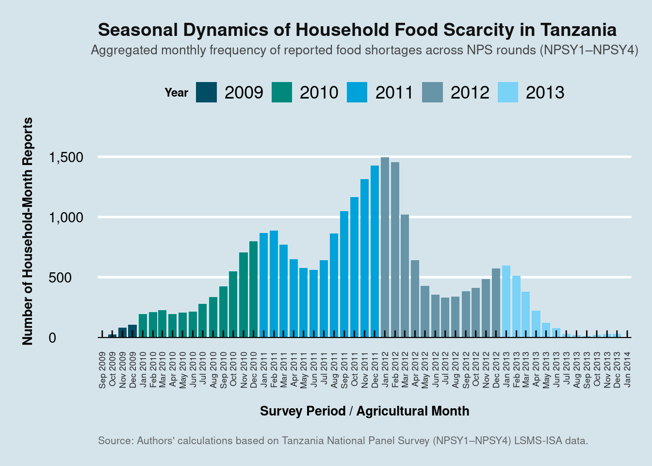
Figure 1 demonstrates that household food shortages in Tanzania follow a predictable bi-modal trajectory. The reported household food scarcity cases peak sharply between November and February. These months also matches the period when the home-grown food reserves are depleted, while the current-season crops remain in immature in the field. The other notable pattern is observed between the months of May and August, when the reported scarcity drops to its lowest annual levels. This also coincides with the harvesting season from the long-rain crop.
To understand the root causes of the observed seasonality, I pool and summarize the prominent drivers by month into primary driver (the first reported cause of scarcity); secondary driver (the second reported cause of scarcity); and tertiary driver (the third reported cause of scarcity).
shocks_long <- raw_data |>
  select(UPHI, round, hh_08, hh_12_1, hh_12_2, hh_12_3) |>
  filter(!is.na(hh_08) & hh_08 %in% c("YES", "Yes", "1")) |>
  rename(
    household_id = UPHI,
    wave = round
  ) |>

  # Pivot 1st, 2nd, and 3rd cause ranks to long format
  pivot_longer(
    cols = c(hh_12_1, hh_12_2, hh_12_3),
    names_to = "cause_rank",
    values_to = "cause_code"
  ) |>
  filter(!is.na(cause_code) & cause_code != "" & cause_code != "96") |>
  mutate(
    # Format cause rank indicator
    cause_rank = case_when(
      cause_rank == "hh_12_1" ~ "Primary Cause",
      cause_rank == "hh_12_2" ~ "Secondary Cause",
      cause_rank == "hh_12_3" ~ "Tertiary Cause"
    ),

    # Cleaning the descriptions descriptions
    shock_description = case_when(
      cause_code %in% c(1, "1",
                        "INADEQUATE HOUSEHOLD STOCKS DUE TO DROUGHT/POOR RAINS") ~
        "Drought / Poor Rains",
      cause_code %in% c(2, "2",
                        "INADEQUATE HOUSEHOLD FOOD STOCKS DUE TO CROP PEST DAMAGE") ~
        "Crop Pest Damage",
      cause_code %in% c(3, "3",
                        "INADEQUATE HOUSEHOLD FOOD STOCKS DUE TO SMALL LAND SIZE") ~
        "Small Land Size",
      cause_code %in% c(4, "4",
                        "INADEQUATE HOUSEHOLD FOOD STOCKS DUE TO LACK OF FARM INPUTS") ~
        "Lack of Farm Inputs",
      cause_code %in% c(5, "5",
                        "FOOD IN THE MARKET WAS VERY EXPENSIVE") ~
        "Expensive Food in Market",
      cause_code %in% c(6, "6",
                        "UNABLE TO REACH THE MARKET DUE TO HIGH TRANSPORTATION COSTS") ~
        "High Transport Costs",
      cause_code %in% c(7, "7", "NO FOOD IN THE MARKET") ~ "No Food in Market",
      cause_code %in% c(8, "8", "FLOODS/WATER LOGGING/HAILSTORM") ~ "Floods / Hailstorm",
      cause_code %in% c(9, "9", "NO MONEY") ~ "No Money / Lack of Funds",
      cause_code %in% c(10, "10", "OTHER (SPECIFY)") ~ "Other Causes",
      TRUE ~ "Other"
    ),

    # Group into macro-typologies
    shock_typology = case_when(
      shock_description %in% c("Drought / Poor Rains",
                               "Floods / Hailstorm",
                               "Crop Pest Damage") ~
        "Agro-Climatic",
      shock_description %in% c("No Money / Lack of Funds") ~
        "Financial & Income Shock",
      shock_description %in% c("Expensive Food in Market",
                               "High Transport Costs",
                               "No Food in Market") ~
        "Market & Price Shock",
      shock_description %in% c("Small Land Size",
                               "Lack of Farm Inputs") ~
        "Production & Input Constraint",
      TRUE ~ "Other"
    )
  )

# -------------------------------------------------------------------------
# Join temp_mapping_formatted with shocks_long
# -------------------------------------------------------------------------
combined_shocks <- temp_mapping_formatted |>
  inner_join(shocks_long, by = c("household_id", "wave"), relationship = "many-to-many")

# -------------------------------------------------------------------------
# Seasonal Profile of Food Scarcity Drivers in Tanzania
# -------------------------------------------------------------------------
monthly_shock_profile <- combined_shocks |>
  mutate(month = month(date, label = TRUE, abbr = TRUE)) |>

  count(month, cause_rank, shock_description) |>

  group_by(month, cause_rank) |>
  slice_max(order_by = n, n = 1, with_ties = FALSE) |>
  ungroup() |>

  mutate(cause_rank = factor(cause_rank, levels = c("Primary Cause", "Secondary Cause", "Tertiary Cause"))) |>

  pivot_wider(
    id_cols = month,
    names_from = cause_rank,
    values_from = shock_description,
    values_fill = "None Reported",
    names_expand = TRUE
  ) |>

  # Order chronologically from Jan to Dec
  arrange(month)

# -------------------------------------------------------------------------
# Rendering the table summary
# -------------------------------------------------------------------------
monthly_shock_gt <- monthly_shock_profile |>
  gt(rowname_col = "month") |>

  # Title and Subtitle
  tab_header(
    title = md("**Seasonal Profile of Food Scarcity Drivers in Tanzania**"),
    subtitle = "Most prevalent primary, secondary, and tertiary drivers by calendar month (Pooled 2009–2013)"
  ) |>

  # Relabel Column Headers
  cols_label(
    `Primary Cause`   = "Primary Driver",
    `Secondary Cause` = "Secondary Driver",
    `Tertiary Cause`  = "Tertiary Driver"
  ) |>

  # Align text
  cols_align(align = "left", columns = everything()) |>

  # Apply Economist-style typography and styling
  tab_options(
    table.font.name                 = "Georgia",
    table.font.size                 = px(12),
    table.width = pct(100),
    heading.align                   = "left",
    heading.title.font.size         = px(16),
    heading.subtitle.font.size      = px(11),
    column_labels.font.weight       = "bold",
    column_labels.background.color  = "#F4F5F7",
    table.border.top.color          = "#111111",
    table.border.top.width          = px(2),
    table.border.bottom.color       = "#111111",
    table.border.bottom.width       = px(2),
    table_body.hlines.color         = "#E0E0E0",
    table_body.hlines.style         = "solid"
  ) |>

  # Add Footnote
  tab_footnote(
    footnote = "Source: Tanzania National Panel Survey (NPS) Household Shock Modules (NPSY1–NPSY4).",
    locations = cells_title(groups = "subtitle")
  )

# Dispay table
monthly_shock_gt| Seasonal Profile of Food Scarcity Drivers in Tanzania | |||
| Most prevalent primary, secondary, and tertiary drivers by calendar month (Pooled 2009–2013)1 | |||
| Primary Driver | Secondary Driver | Tertiary Driver | |
|---|---|---|---|
| Jan | Drought / Poor Rains | No Money / Lack of Funds | No Money / Lack of Funds |
| Feb | Drought / Poor Rains | No Money / Lack of Funds | No Money / Lack of Funds |
| Mar | Drought / Poor Rains | No Money / Lack of Funds | No Money / Lack of Funds |
| Apr | Drought / Poor Rains | No Money / Lack of Funds | No Money / Lack of Funds |
| May | Drought / Poor Rains | No Money / Lack of Funds | No Money / Lack of Funds |
| Jun | Drought / Poor Rains | No Money / Lack of Funds | No Money / Lack of Funds |
| Jul | Drought / Poor Rains | No Money / Lack of Funds | No Money / Lack of Funds |
| Aug | Drought / Poor Rains | No Money / Lack of Funds | No Money / Lack of Funds |
| Sep | Drought / Poor Rains | No Money / Lack of Funds | No Money / Lack of Funds |
| Oct | Drought / Poor Rains | No Money / Lack of Funds | No Money / Lack of Funds |
| Nov | Drought / Poor Rains | No Money / Lack of Funds | No Money / Lack of Funds |
| Dec | Drought / Poor Rains | No Money / Lack of Funds | No Money / Lack of Funds |
| 1 Source: Tanzania National Panel Survey (NPS) Household Shock Modules (NPSY1–NPSY4). | |||
As documented in Table 1, “Drought/Poor rains” is identified as the single leading primary cause of food scarcity across 11 out of 12 calendar months, reaffirming that crop production failures remain the single largest direct threat to food security. In June, “No Money / Lack of Funds” displaces drought as the primary driver of scarcity. June marks the onset of main crop harvesting; while physical food becomes available in fields, households experience extreme cash liquidity shortages due to immediate financial demands (e.g., labor costs, debt settlements, and land rental fees).
“No Money / Lack of Funds” occupies 100% of the secondary and tertiary driver positions across every single month. This demonstrates that cash constraints permanently erode household resilience, preventing families from purchasing food from local markets when harvest yields fail.
When confronted with food shortages, households adopt short-term behavioral coping mechanisms to manage dietary deficits.
# -------------------------------------------------------------------------
# Coping Module & Calculate rCSI + Behavioral Flags
# -------------------------------------------------------------------------
coping_analysis <- raw_data |>
  # Select key indicators from the dictionary
  select(
    UPHI, round,
    hh_01,
    hh_02_1, hh_02_2, hh_02_3, hh_02_4,
    hh_02_5, hh_02_6, hh_02_7, hh_02_8
  ) |>

  mutate(across(starts_with("hh_02_"), ~ ifelse(is.na(.) | . < 0, 0, as.numeric(.)))) |>

  # Calculate Standard Reduced Coping Strategies Index (rCSI)
  # Standard WFP Weights: Less preferred (1), Borrow food (2), Limit portions (1), Restrict adults (3), Reduce meals (1)
  mutate(
    rCSI = (hh_02_1 * 1) +
           (hh_02_6 * 2) +
           (hh_02_3 * 1) +
           (hh_02_5 * 3) +
           (hh_02_4 * 1),

    # Binary flags for whether a strategy was used at least 1 day in the past week
    worried_food            = ifelse(hh_01 %in% c("YES", "Yes", 1, "1"), 1, 0),
    relied_less_preferred  = ifelse(hh_02_1 > 0, 1, 0),
    limited_variety         = ifelse(hh_02_2 > 0, 1, 0),
    limited_portions        = ifelse(hh_02_3 > 0, 1, 0),
    reduced_meals           = ifelse(hh_02_4 > 0, 1, 0),
    adult_sacrifice_child   = ifelse(hh_02_5 > 0, 1, 0),
    borrowed_food           = ifelse(hh_02_6 > 0, 1, 0),
    no_food_in_house        = ifelse(hh_02_7 > 0, 1, 0),
    went_day_night_fasting  = ifelse(hh_02_8 > 0, 1, 0)
  )

# -------------------------------------------------------------------------
# Coping Profile across Survey Waves / Shock States
# -------------------------------------------------------------------------
coping_summary <- coping_analysis |>
  group_by(round) |>
  summarise(
    `Sample Size (N)`                = n(),
    `Worried About Food (%)`         = mean(worried_food, na.rm = TRUE) * 100,
    `Mean rCSI Score`                = mean(rCSI, na.rm = TRUE),
    `Rely on Less Preferred (%)`     = mean(relied_less_preferred, na.rm = TRUE) * 100,
    `Limit Portion Size (%)`         = mean(limited_portions, na.rm = TRUE) * 100,
    `Reduce Meals Per Day (%)`       = mean(reduced_meals, na.rm = TRUE) * 100,
    `Adults Restrict for Kids (%)`   = mean(adult_sacrifice_child, na.rm = TRUE) * 100,
    `Borrow Food / Rely on Kin (%)`  = mean(borrowed_food, na.rm = TRUE) * 100,
    `Whole Day Fasting (%)`          = mean(went_day_night_fasting, na.rm = TRUE) * 100
  )

# -------------------------------------------------------------------------
# Summaries
# -------------------------------------------------------------------------
coping_gt <- coping_summary |>
  gt(rowname_col = "round") |>
  tab_header(
    title = md("**Short-Term Household Coping Profile**"),
    subtitle = "Prevalence of 7-day coping strategies and mean rCSI scores across survey waves"
  ) |>
  fmt_number(
    columns = c(`Mean rCSI Score`),
    decimals = 2
  ) |>
  fmt_number(
    columns = contains("(%)"),
    decimals = 1
  ) |>
  cols_align(align = "center", columns = everything()) |>
  tab_options(
    table.font.name               = "Georgia",
    table.font.size               = px(12),
    heading.align                 = "left",
    heading.title.font.size       = px(16),
    heading.subtitle.font.size    = px(11),
    column_labels.font.weight     = "bold",
    column_labels.background.color= "#F4F5F7",
    table.border.top.color        = "#111111",
    table.border.top.width        = px(2),
    table.border.bottom.color     = "#111111",
    table.border.bottom.width     = px(2)
  ) |>
  tab_footnote(
    footnote = "Source: Tanzania National Panel Survey (NPS) Module 2 (7-Day Food Security & Coping).",
    locations = cells_title(groups = "subtitle")
  )

coping_gt| Short-Term Household Coping Profile | |||||||||
| Prevalence of 7-day coping strategies and mean rCSI scores across survey waves1 | |||||||||
| Sample Size (N) | Worried About Food (%) | Mean rCSI Score | Rely on Less Preferred (%) | Limit Portion Size (%) | Reduce Meals Per Day (%) | Adults Restrict for Kids (%) | Borrow Food / Rely on Kin (%) | Whole Day Fasting (%) | |
|---|---|---|---|---|---|---|---|---|---|
| 2 | 8163 | 34.0 | 3.43 | 29.5 | 14.4 | 21.9 | 7.3 | 9.8 | 3.1 |
| 3 | 9998 | 30.2 | 3.14 | 26.1 | 12.6 | 18.6 | 6.0 | 8.8 | 2.8 |
| 4 | 4961 | 31.2 | 3.06 | 26.5 | 12.9 | 19.1 | 6.3 | 9.8 | 2.9 |
| 1 Source: Tanzania National Panel Survey (NPS) Module 2 (7-Day Food Security & Coping). | |||||||||
Food anxiety affects roughly one-third of households in each wave, peaking at 34.0% in Wave 2 before stabilizing at 31.2% in Wave 4 Table 2. The mean reduced Coping Strategies Index (rCSI) score improved moderately over time, declining from 3.43 in Wave 2 to 3.06 in Wave 4. Modifying dietary quality (Relying on Less Preferred Foods, 26.5%–29.5%) and restricting meal frequency (Reducing Meals Per Day, 18.6%–21.9%) are the primary frontline responses. Severe distress behaviors, such as Whole Day Fasting (2.8%–3.1%) and Adults Restricting Intake for Children (6.0%–7.3%), remain persistent among the most vulnerable sub-populations.
Looking at the findings, I make the following conclusion and propose the next three policy recommendations:
These phenomena can be addressed through three main policy perspectives:
First, social protection programs need to align strictly with the lean season identified in Figure 1. Disbursing assistance between October and November (prior to the peak shortage months) might provide maximum buffering capacity.
Next, the emergence of “No Money / Lack of Funds” as the primary driver in June (see Table 1) demonstrates a need for post-harvest liquidity solutions. Expanding access to micro-credit, warehouse receipt systems, and harvest financing can prevent households from engaging in premature distress sales of early crops.
Finally, because cash poverty permanently underpins climate shocks Table 2, climate adaptation strategies (e.g., drought-resistant seeds, small-scale irrigation) need to be bundled with village savings and loans and financial inclusion initiatives.